Batch noramlization은 이전 residual block과 함께 딥러닝 모델의 convergence를 가능하게 하고 많은 layer를 규치적으로 학습할 수 있게 한다. 다음과 같은 문제를 다룰 수 있는 technique이다.
1) 데이터 전처리 방식에 따라 모델의 결과는 큰 차이를 가진다. 정규화 사용여부 등이 있다.
2) MLP나 CNN에서의 중간 layer에서 variable들은 layer의 input 부터 output까지, 같은 layer 내의 다른 unit 등 매우 다양한 값을 가진다. 이런 넓은 분포의 variable들 모델의 convergence를 어렵게 한다.
3) 깊은 딥러닝 모델들은 복잡하고 오버피팅이 일어나기 쉽다. regularization이 중요한 이유이기도 하다.
Batch norm은 각각의 layer에 선택적으로 적용되는데, 먼저 input data에 대해 표준화하고 scale coefficient, scale offset을 적용한다. 이 과정이 batch 단위로 이루어지기에 이렇게 명명되었고 당연히 minibatch size가 1일 때는 그 효과가 드러나지 않는다. 따라서 batch size를 결정하는 것은 batch norm을 수행할 때 더욱 중요해지는데 minibatch B에서 batch norm의 하나의 input을 x라 한다면 다음과 같이 표현된다.
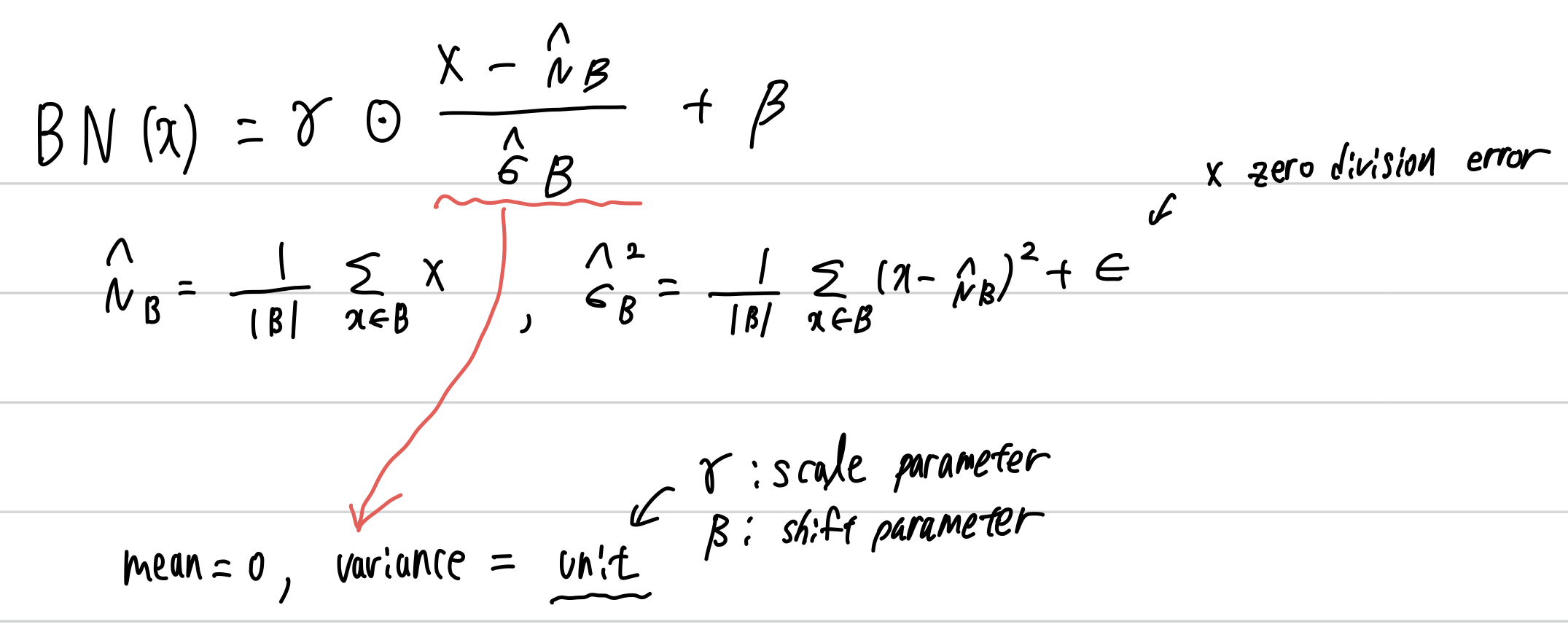
이런 작업을 거치게 된다면 variable의 다양한 크기로 인한 diergence가 없어지고 상대적으로 더 다양한 learning rate을 사용해 볼 수 있다. 또한 위에서 std에 더한 noise는 scaling을 방해하는 것이 아닌가라고 생각할 수 있지만 학습에서 이점을 가진다. optimization에서 다뤘던 내용과 같은 이유로 더 빠르게 학습이 가능하고 더 적은 오버피팅 확률을 갖게 된다.
다시 생각해보면 위 bn은 전체 데이터셋에 대해 mean과 variance를 구하고 그 값으로 표준화하는 것이 가장 이상적일 것이다. 하지만 훈련 중 이런 연산은 intermediate variable에 대해 모두 그리고 update 마다 변화하는 모든 data에 대해 수행하는 것은 불가능하다. 하지만 model이 훈련되고 난 이후에는 각 layer에 대해 전체 데이터셋 기준으로 mean과 variance는 구할 수 있다. 따라서 training mode에서는 normalizing by minibatch statistics, prediction mode에서는 normalizing by dataset statistics로 다르게 표준화를 실시한다.
훈련 전후 차이 뿐만 아니라 bn은 conv layer와 fc layer에서도 다르게 이뤄진다. 이 이유는 bn이 full minibatch에 대해 한번에 이뤄지기에 batch 차원을 고려해야 하기 때문이다.
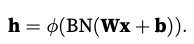
1) fc layer : affine transformation 이후, activation function 이전
2) conv layer : conv 이후, activation function 이전 + conv가 다수의 채널을 가질 경우 bn이 각각의 채널의 결과에 대해 모두 수행되어져야 함. m(# of examples of minibatch) x p(height of the output of conv) x q(width of the output of conv) 개의 요소에 대해 모두 수행햐야 하고 이는 모든 spatial location에 대해 bn 연산을 하는 것이다.
다시 훈련 전후에 따른 차이에 집중해본다면, 훈련이 종료된 이후 예측 과정에서의 bn에서는 더 이상 noise를 반영할 필요가 없고 훈련 전에 수행하던 per batch normalization이 필요 없고 예측을 한번 하게 되면 그 때만 bn 연산을 하면 된다.
코드로 구현하면 다음과 같다.
def batch_norm(X, gamma, beta, moving_mean, moving_var, eps, momentum):
    # Use `is_grad_enabled` to determine whether the current mode is training
    # mode or prediction mode
    if not torch.is_grad_enabled():
        # If it is prediction mode, directly use the mean and variance
        # obtained by moving average
        X_hat = (X - moving_mean) / torch.sqrt(moving_var + eps)
    else:
        assert len(X.shape) in (2, 4)
        if len(X.shape) == 2:
            # When using a fully-connected layer, calculate the mean and
            # variance on the feature dimension
            mean = X.mean(dim=0)
            var = ((X - mean) ** 2).mean(dim=0)
        else:
            # When using a two-dimensional convolutional layer, calculate the
            # mean and variance on the channel dimension (axis=1). Here we
            # need to maintain the shape of `X`, so that the broadcasting
            # operation can be carried out later
            mean = X.mean(dim=(0, 2, 3), keepdim=True)
            var = ((X - mean) ** 2).mean(dim=(0, 2, 3), keepdim=True)
        # In training mode, the current mean and variance are used for the
        # standardization
        X_hat = (X - mean) / torch.sqrt(var + eps)
        # Update the mean and variance using moving average
        moving_mean = momentum * moving_mean + (1.0 - momentum) * mean
        moving_var = momentum * moving_var + (1.0 - momentum) * var
    Y = gamma * X_hat + beta  # Scale and shift
    return Y, moving_mean.data, moving_var.data
조금 더 정제하여 그 기능을 구현한 코드는 다음과 같다.
class BatchNorm(nn.Module):
    # `num_features`: the number of outputs for a fully-connected layer
    # or the number of output channels for a convolutional layer. `num_dims`:
    # 2 for a fully-connected layer and 4 for a convolutional layer
    def __init__(self, num_features, num_dims):
        super().__init__()
        if num_dims == 2:
            shape = (1, num_features)
        else:
            shape = (1, num_features, 1, 1)
        # The scale parameter and the shift parameter (model parameters) are
        # initialized to 1 and 0, respectively
        self.gamma = nn.Parameter(torch.ones(shape))
        self.beta = nn.Parameter(torch.zeros(shape))
        # The variables that are not model parameters are initialized to 0 and 1
        self.moving_mean = torch.zeros(shape)
        self.moving_var = torch.ones(shape)
    def forward(self, X):
        # If `X` is not on the main memory, copy `moving_mean` and
        # `moving_var` to the device where `X` is located
        if self.moving_mean.device != X.device:
            self.moving_mean = self.moving_mean.to(X.device)
            self.moving_var = self.moving_var.to(X.device)
        # Save the updated `moving_mean` and `moving_var`
        Y, self.moving_mean, self.moving_var = batch_norm(
            X, self.gamma, self.beta, self.moving_mean,
            self.moving_var, eps=1e-5, momentum=0.9)
        return Y
이렇게 배운 batch normalization을 이전에 배운 LeNet에 적용해보자.
위에서 말했듯, conv 연산 이후에 그리고 activiation 이전에 bn을 수행한다.
net = nn.Sequential(
    nn.Conv2d(1, 6, kernel_size=5), BatchNorm(6, num_dims=4), nn.Sigmoid(),
    nn.AvgPool2d(kernel_size=2, stride=2),
    nn.Conv2d(6, 16, kernel_size=5), BatchNorm(16, num_dims=4), nn.Sigmoid(),
    nn.AvgPool2d(kernel_size=2, stride=2), nn.Flatten(),
    nn.Linear(16*4*4, 120), BatchNorm(120, num_dims=2), nn.Sigmoid(),
    nn.Linear(120, 84), BatchNorm(84, num_dims=2), nn.Sigmoid(),
    nn.Linear(84, 10))
lr, num_epochs, batch_size = 1.0, 10, 256
train_iter, test_iter = d2l.load_data_fashion_mnist(batch_size)
d2l.train_ch6(net, train_iter, test_iter, num_epochs, lr, d2l.try_gpu())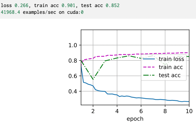
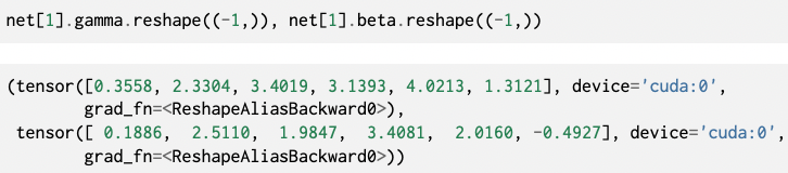
scale parameter gamma와 shift parameter beta에 대해서도 학습된 결과를 알 수 있다. 아래는 첫번째 bn layer 결과를 불러온 것이다.
bn도 당연히 torch 모듈에서 사용 가능하고 위 코드를 다름과 같이 모듈을 사용해 더 간단하게 구현할 수 있다.
net = nn.Sequential(
    nn.Conv2d(1, 6, kernel_size=5), nn.BatchNorm2d(6), nn.Sigmoid(),
    nn.AvgPool2d(kernel_size=2, stride=2),
    nn.Conv2d(6, 16, kernel_size=5), nn.BatchNorm2d(16), nn.Sigmoid(),
    nn.AvgPool2d(kernel_size=2, stride=2), nn.Flatten(),
    nn.Linear(256, 120), nn.BatchNorm1d(120), nn.Sigmoid(),
    nn.Linear(120, 84), nn.BatchNorm1d(84), nn.Sigmoid(),
    nn.Linear(84, 10))